The Performance and Efficiency of Flat Plate Collectors with Different Absorbers and Different Convection Heat Loss Levels
Introduction
The flat plate collectors are still among the most popular devices to intercept and exploit solar energy. The absorbed solar energy is transferred to a fluid passing in contact with its absorber plate.
Increasing the efficiency of such a device has aroused the interest of many investigators.1-8
The main part of such a system is its absorber plate whose thermal performance affects essentially its efficiency.
To study the thermal response of the collector one has to get information on the incident global solar irradiance q (t), W/m2 and its variation along the local day time.
This represents an essential input parameter to study the performance theoretically.
Several trials are made to predict the function q (t).9-17
In the present study q (t)9 is considered.
Absorbers of different material such as: Copper, Aluminum, Steel, Glass and Mica are treated.
Water is considered in the present study as the working fluid.
Other factors affect the efficiency of the collector as the water rate of flow, selective coatings of the front surface of the absorber, heat losses by convection and radiation, the surface absorptivity of the surface.
Heating Problem
In setting up the problem it is assumed that the solar insolation q (t) W/m2 is received on the upper surface of the absorber plate, where it will be partly reflected and partly absorbed (1-R) q (t) W/m2. The absorbed energy will induce heating effects within the absorber. This part of heat energy will be transferred to the working fluid glazing its near surface.
A thin absorber is considered in this study thus neglecting any temperature gradient across its thickness.
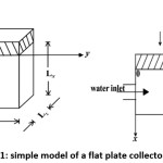
A simple device for the collector is shown in fig. (1). The absorber is kept in a horizontal position. The problem is thus treated as one dimensional problem.16, 18
Figure 1: Simple model of a flat plate collector.
The accepted distribution q (t)9 has the form:

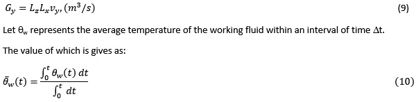
It is a symmetrical distribution about the midday time t0 = tmax = td/2 with maximum irradiance qmax, W/m2 at t = tmax, where td is the length of the solar day. The value of “td” is given in terms of the latitude “L” and the solar declination “δ”19 as follows:
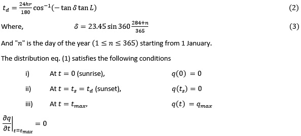
Determination of the temperature of the absorber.
To find the temperature absorber, let us write the heat balance equation in the form:

The first term represents the heat energy absorbed by the absorber, “R” is the reflectance of the front surface, “h”, (W/m2K) is the heat transfer by convection at the front surface, “δ”, (kg/m3) is the density of the absorber material, “l”, (m) is thickness of the absorber, and Θ(t) = (T – T0) is the excess temperature relative to the ambient temperature “T0”.
Heat losses due to radiation (infrared emission) are neglected. Equation (4) has an integrating factor:
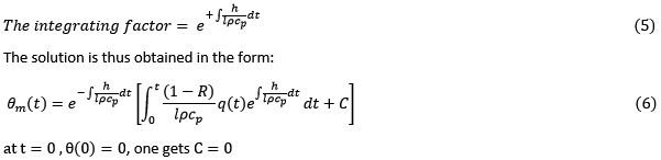
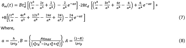
Substituting the distribution equation (1) in equation (6) and performing the included integration, one gets the solution for q(t) expressed as follows:
Determination of the temperature of the working fluid temperature:
Let the thin absorber of thickness “l”, (m) represents the upper ceiling for a reservoir of dimensions Lx, Ly and Lz,
(m). The upper surface of the thin absorber of area Sx = Ly Lz, (m2) is subjected to the incident solar radiation q(t), W/m2.
The x-axis is taken vertically downwards. It is coincident with the direction of the incident radiation. The volume of the absorber material is Vabs = lmLyLz, m3. The volume of the reservoir is Vres = LxLyLz, m3.
The sides of the reservoir are assumed to be thermally insulated. The working fluid enters the reservoir from the faced Sy = Lz Lx, (m2) and emerges from the opposite sides. For simplicity, let Ly = Lz = 1m.
The fluid flows along the y-direction with velocity vy,(m/s), and volumetric rate:
Thus, the heat balance equation concerning the working fluid within an interval of time Δt is written in the form:
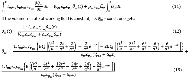
The first term on the right-hand side of equation (11) represents the heat energy stored in the working fluid within the reservoir. In an interval of time Δt. The second term represents the heat energy gained by the flowing fluid during the same interval Δt, s.
The efficiency η:
The efficiency of the flat plate collector within a certain interval of time Δt = ∫0t dt, s, is defined through the equation:
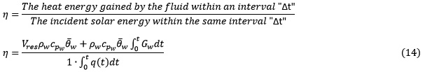
Substituting the distribution equation (1) in equation (14) and performing the included integration, one gets the efficiency expressed as follows :
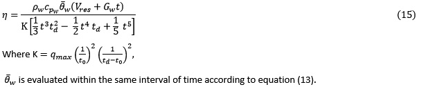
Computations
The experimental values of the incident solar irradiance received per unit area in Makah9 with parameters: qmax = 938 W/m2, td = 12 hr, These values are computed according to our model (eq.1). The obtained fitting between them is revealed to be 92%.
Two cooling conditions are considered h=3 W/m2 K and h=10 W/m2 K the reflection coefficient R = 0.2. Five materials are considered. These are Copper (Cu), Aluminum (Al), Steel, Crown glass and Mica. The physical parameters of which are given in table (1).
Table 1: The physical parameters of the considered absorber materials.20
|
Element
|
ρ, kg/m3
|
Cp, J/kg. K
|
|
Cu
|
8954
|
383.1
|
|
Al
|
2710
|
910
|
|
Mica
|
2883
|
880
|
|
Steel
|
7833
|
465
|
|
Crown glass
|
2500
|
670
|
For water as the working fluid: ρw = 1000 kg/m3, cp w = 4.1818 x 1.3 J/kg K The volumetric water rate Gw y = 10-7 m3/s and the volume of the reservoir Vres = 0.05 m3
The temperature Θ (t) of the absorber plate:
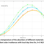
The temperature of the five elements subjected to the incident solar radiation q(t)9 is computed along the local day time according to equation (7). Shifted time is considered according to which the sunrise time “tr” is taken as zero, i.e. tr = 0. The thickness of the absorber for each case is taken as lm = 0/01m. The obtained results are given in table (2) and table (3) for h=3 W/m2 K and h=10 W/m2 K respectively. These data are illustrated graphically in figures (2) and (3) respectively.
Table 2: The variation of the temperature of the absorbers of different materials subjected to incident solar radiation for h=3 W/m2 K
|
Local time, hr
|
Shifted time ť, hr.
|
Θm(t), K
|
|
Cu
|
Al
|
Mica
|
Steel
|
Crown glass
|
|
6.5
|
0
|
0
|
0
|
0
|
0
|
0
|
|
7.5
|
1
|
0. 5
|
3.27
|
3.36
|
2.03
|
4.54
|
|
8.5
|
2
|
12.5
|
20
|
20
|
14.1
|
27
|
|
9.9
|
3
|
38.4
|
52.3
|
51.9
|
38.7
|
67.7
|
|
10.5
|
4
|
73.7
|
94.8
|
94
|
72.7
|
118
|
|
11.5
|
5
|
113
|
139
|
138
|
110
|
167
|
|
12.5
|
6
|
148
|
177
|
176
|
145
|
205
|
|
13.5
|
7
|
173
|
201
|
200
|
171
|
224
|
|
14.5
|
8
|
185
|
207
|
207
|
183
|
221
|
|
15.5
|
9
|
180
|
193
|
194
|
179
|
196
|
|
16.5
|
10
|
160
|
162
|
164
|
160
|
153
|
|
17.5
|
11
|
129
|
121
|
124
|
131
|
102
|
|
18.5
|
12
|
95.2
|
80.5
|
83.7
|
99.2
|
56.9
|
Figure 2: The temperature of the absorbers of different materials subjected to incident solar irradiances with local day time for, h=3 W/m2 K
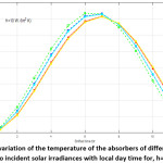
Table 3: The variation of the temperature of the absorbers of different materials subjected to incident solar radiation for h=10 W/m2 K
|
Local time ť, hr.
|
Shifted time ť, hr.
|
Θw(t), K
|
|
Cu
|
Al
|
Mica
|
Steel
|
Crown glass
|
|
6.5
|
0
|
0
|
0
|
0
|
0
|
0
|
|
7.5
|
1
|
1.99
|
2.55
|
2.5
|
1.91
|
3.28
|
|
8.5
|
2
|
11.1
|
13.3
|
13.1
|
10.7
|
15.7
|
|
9.5
|
3
|
26.1
|
30
|
29.6
|
25.5
|
33.5
|
|
10.5
|
4
|
43.2
|
47.8
|
47.4
|
42.4
|
51.6
|
|
11.5
|
5
|
58.4
|
62.7
|
62.3
|
57.6
|
65.8
|
|
12.5
|
6
|
68.4
|
71.6
|
71.3
|
67.9
|
73.4
|
|
13.5
|
7
|
71.5
|
73
|
72.8
|
71.3
|
73
|
|
14.5
|
8
|
66.9
|
66.4
|
66.4
|
67.2
|
64.8
|
|
15.5
|
9
|
55.6
|
53.2
|
53.4
|
56.2
|
50.2
|
|
16.5
|
10
|
39.5
|
35.8
|
36
|
40.4
|
31.9
|
|
17.5
|
11
|
22.4
|
18.1
|
18.4
|
23.4
|
14.3
|
|
18.5
|
12
|
9.02
|
5.48
|
5.7
|
9.87
|
2.84
|
Figure 3: The variation of the temperature of the absorbers of different materials subjected to incident solar irradiances with local day time for, h=10 W/m2 K
The temperature of the working fluid:
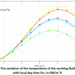
The temperature of the working fluid (water) qw is computed according to equation (13). The heat transfer coefficient for convection “H” is taken equal to 3 W/m2 K. The obtained results for the considered five elements Cu, Al, Steel, Crown glass and Mica are given in table (4). And are illustrated graphically in figure (4).
Table 4: The variation of the temperature of the working fluid qw, 0K with local day time for [h = 3 W / m2 K]
|
Local time ť, hr.
|
Shifted time ť, hr.
|
Θw, 0K
|
|
Cu
|
Al
|
Mica
|
Steel
|
Crown glass
|
|
6.5
|
0
|
0
|
0
|
0
|
0
|
0
|
|
7.5
|
1
|
0. 08
|
0.39
|
0.41
|
0.39
|
0.36
|
|
8.5
|
2
|
2.05
|
2.36
|
2.43
|
2.46
|
2.16
|
|
9.5
|
3
|
6.29
|
6.17
|
6.30
|
6.74
|
5.42
|
|
10.5
|
4
|
12.09
|
11.2
|
11.40
|
12.70
|
9.45
|
|
11.5
|
5
|
18.54
|
16.40
|
16.80
|
19.20
|
13.40
|
|
12.5
|
6
|
24.28
|
20.90
|
21.40
|
25.30
|
16.4
|
|
13.5
|
7
|
28.38
|
23.70
|
24.30
|
29.70
|
18.00
|
|
14.5
|
8
|
30.35
|
24.40
|
25.10
|
31.80
|
17.70
|
|
15.5
|
9
|
29.53
|
22.70
|
23.50
|
31.20
|
15.70
|
|
16.5
|
10
|
26.25
|
19.10
|
19.90
|
27.90
|
12.20
|
|
17.5
|
11
|
21.16
|
14.30
|
150
|
22.80
|
8.18
|
|
18.5
|
12
|
15.62
|
9.50
|
10.20
|
17.30
|
4.56
|
Figure 4: The variation of the temperature of the working fluid qw (t), K, with local day time for, h=3W/m2 K
The Efficiency (η) Computations
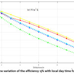
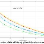
The efficiency is computed according to equation (15) for the five elements for different time intervals along the local day time. The obtained results are given in table (5) and table (6) for and , respectively. These data are illustrated graphically in figures (5) and (6) respectively.
Table 5: The variation of the efficiency η with local day time for [h = 3 W / m2 K]
|
Shifted time ť, hr.
|
η%
|
|
Cu
|
Al
|
Mica
|
Steel
|
Crown glass
|
|
1
|
68
|
73
|
77.58
|
67.1
|
70.89
|
|
2
|
65
|
64.38
|
66.15
|
67.1
|
58.9
|
|
3
|
58.9
|
57.7
|
58.85
|
62.98
|
50.64
|
|
4
|
55.7
|
51.57
|
52.57
|
58.34
|
43.58
|
|
5
|
51.7
|
45.85
|
46.79
|
53.63
|
37.37
|
|
6
|
46.9
|
40.40
|
41.32
|
48.86
|
31.76
|
|
7
|
42.03
|
35.11
|
36
|
43.99
|
26.58
|
|
8
|
37.2
|
29.85
|
30.72
|
38.94
|
21.66
|
|
9
|
31.9
|
24.55
|
25.38
|
33.63
|
16.90
|
|
10
|
26.3
|
19.18
|
19.96
|
28.01
|
12.28
|
|
11
|
20.58
|
13.88
|
14.6
|
22.21
|
7.95
|
|
12
|
15.1
|
9.19
|
9.82
|
16.72
|
4.41
|
Figure 5: The variation of the efficiency η% with local day time for h=3 W/m2 K
Table 6: The variation of the efficiency η with local day time for [ h=10 W / m2 K]
|
Shifted time ť, hr.
|
η%
|
|
Cu
|
Al
|
Mica
|
Steel
|
Crown glass
|
|
1
|
62.08
|
73
|
77.58
|
63.27
|
70.89
|
|
2
|
49.63
|
64.38
|
66.15
|
50.81
|
58.9
|
|
3
|
40.02
|
57.7
|
58.85
|
41.52
|
50.64
|
|
4
|
32.67
|
51.57
|
52.57
|
34.05
|
43.58
|
|
5
|
26.74
|
45.85
|
46.79
|
28
|
37.37
|
|
6
|
21.71
|
40.40
|
41.32
|
22.89
|
31.76
|
|
7
|
17.37
|
35.11
|
36
|
18.39
|
26.58
|
|
8
|
13.43
|
29.85
|
30.72
|
14.33
|
21.66
|
|
9
|
9.84
|
24.55
|
25.38
|
10.56
|
16.90
|
|
10
|
6.5
|
19.18
|
19.96
|
7.06
|
12.28
|
|
11
|
3.57
|
13.88
|
14.6
|
3.96
|
7.95
|
|
12
|
1.43
|
9.19
|
9.82
|
1.66
|
4.41
|
Figure 6: The variation of the efficiency η% with local day time for h=10 W/m2 K
Conclusions
The obtained results make it possible to formulate a set of conclusions:
1- The temperature of the thin absorber Θt does depend linearly on the maximum value of the received incident solar irradiance qmax, W/m2.
2- The function Θt changes with the local exposure time and passes through a maximum value at critical time that differs with cooling conditions.
3- The value of Θt depends on the physical parameters of the absorber material. The curves of Θt for the two elements Al, Mica are nearly coincident also for Cu & steel. This indicates that the dependence on the physical parameter is not the same for all elements higher values of Θt is obtained for glass element. This result is of vital economical importance if one considers the price of the raw materials in relation to the obtained relative efficiencies. Moreover, it depends principally on cooling conditions.
3- The temperature of the working fluid varies with local day time, volume of the reservoir, the volumetric rate of the working fluid, and the geometrical and physical properties of the absorber plate.
4- The efficiency of the collector as given through eq. (15) is inversely proportional to the maximum value of the incident solar irradiance, and it does depend also on all other operating conditions as shown in equation (15).
All such factors are well known, nevertheless, our study represents a quantitative analysis of the flat plate collector dealing with its performance and this may be useful for further analysis.
Acknowledgements
We thank the referees and the editor for their helpful comments and constructive suggestions that greatly improved the presentation of this paper
Funding
This research received no specific grant from any funding agency.
Conflict of Interest
The author has no conflicts of interest to disclose.
References
- G. N. Tiwari, S. Suneja, Solar thermal engineering systems, Narosa publishing house, London, (1997) Ch. 3 P. 82.
- G. M. Nouidu, J. P. Agrawal, A theoretical study of heat transfer in a flat plate collector, solar energy 26, pp.313 (1981).
CrossRef
- L. Jianmin, X. Wenhua, Analysis of thermal performance of a new type of flat-plate collector with a black ceramic absorber, Int. Energy Journal 12(2) (1990).
- S. A. Kalogiron, Solar thermal collectors and applications, Progress in energy and combustion science 30, 231-295 (2004)
CrossRef
- W. E. Buckles, S. A. Klein, Solar energy, vol.35, p417 (1980)
CrossRef
- S. A. Shalaby, A study on flat plate collector, Indian J. Physics 69B (5), pp. 373-388 (1995).
- S. K. Samdarshi, S. C. Mullick, Analysis of the top heat loss factor of flat plate solar collector with single and double glazing. Int. J. Energy Res. Vol.14, p975 (1990).
CrossRef
- D. Gupta, S. C. Solanki, J. S. Saini, Effect of artificial roughness on performance of solar air heaters, New Delhi: Solar Energy society of India/Tata McGraw Hill: (1990) p.14.
- M. K. El-Adawi, Prediction of Symmetrical and Asymmetrical of Diurnal Global Solar Irradiance Distribution – New Approach, Optical and Photonics Journal, 2019,9 ,15-24
CrossRef
- B. Y. Liu, R. C. Jordan, The interrelationship and characteristic distribution of direct, diffuse and total radiation, Solar energy vol.4(1), (1960).
CrossRef
- S. I. Reddy, An empirical method for estimation of the total solar radiation, Solar Energy, vol.13, pp.289 (1971).
CrossRef
- M. M. Munroe, Estimation of irradiance on a horizontal surface from U.K. average meteorological data, Solar Energy vol.24, pp.235 (1980).
CrossRef
- C. T. Leung, The fluctuation of solar irradiance in Hong Kong, Solar Energy vol.25, pp. 485 (1980).
CrossRef
- M. K. El-Adawi, M. M. Al-Nicklawi, A. A. Kutub, G. G. Al-Barakati, Estimation of the hourly solar irradiance on a horizontal surface, Solar Energy vol.36(2), pp.129(1986).
CrossRef
- S. A. Shalaby, Estimation of global solar irradiance on a horizontal surface – New Approach, Indian J. Phys. 68B (6), pp 503-513(1994).
- M. K. El-Adawi, New approach to modelling a flat plate collector Fourier transforms technique, Renewable Energy 26, pp.489-506(2002).
CrossRef
- M. K. El-Adawi, S. A. Shalaby, S. E. S. Abd El-Ghany, F. E. Salman and M. A. Attallah, prediction of the daily global solar irradiance received on a horizontal surface – New approach, Int. Refereed J. of Engineering and Science (IRJES), vol.4 issue 6, pp.85-93, (2015).
- M. K. El- Adawi, On flat plate collector-New approach, Indian J. Phys. 72B (5).505-514(1998).
- J. A. Duffiee, W. A. Beckman, Solar Energy Thermal processes, Wiley-Interscience, New York (1974).
- E. R.G. Eckert and R. M. Drake Analysis of Heat and Mass Transfer (International Student Edition) (Japan: McGraw- hill, Kogakusha Ltd) (1972).

This work is licensed under a Creative Commons Attribution 4.0 International License.