Evaluation of Dielectric Relaxation Parameters from Ionic Thermocurrent Spectrum Involving General Order Kinetics

D. K. Dwivedi

Amorphous Semiconductor Research Lab Department of Physics, M.M.M. University of Technology, Gorakhpur- 273010(India)

Corresponding Author Email: todkdwivedi@gmail.com

DOI : http://dx.doi.org/10.13005/msri/120111

ABSTRACT:

Ionic thermocurrent (ITC) spectrum is much similar to a thermoluminescence (TL) glow curve involving monomolecular kinetics. Like TL processes, it is found that the ITC spectrum involves different orders of kinetics which depends on the experimental conditions of polarization and rate of rapid cooling. In the present work a generalized equation has been developed which is capable of explaining the occurrence of ITC spectrum involving various order of kinetics. Dielectric relaxation parameters, order of kinetics and approximate number of dipoles per unit volume can be evaluated easily using the proposed model.

KEYWORDS: Ionic thermocurrent (ITC); order of kinetics; thermally stimulated processes; dielectric relaxation parameters

Copy the following to cite this article: Dwivedi D. K. Evaluation of Dielectric Relaxation Parameters from Ionic Thermocurrent Spectrum Involving General Order Kinetics. Mat.Sci.Res.India;12(1)

Copy the following to cite this URL: Dwivedi D. K. Evaluation of Dielectric Relaxation Parameters from Ionic Thermocurrent Spectrum Involving General Order Kinetics. Mat.Sci.Res.India;12(1). Available from: http://www.materialsciencejournal.org/?p=2588

Introduction

Thermally stimulated discharge current (TSDC) technique is ideal for the investigation of the structure of polymers, semi-crystalline polymers and co-polymers because it is a more sensitive alternative than other thermal analysis techniques for detecting the transitions that depend on changes in mobility of molecular scale structural units^1-7. The technique can also be applied for the investigation of charge storage and transport processes in high resistivity materials and polymers. For many applications of polymers and doped polymers, it is necessary to know the dielectric properties of material ⁸. Polymer films, which can be polarized in an external electrical field, find applications as sensors sensitive to mechanical vibrations⁹, temperature changes or moisture¹⁰. Further application of doped materials is polymer based field effect transistor sensors¹¹. TSDC is quite useful for the study of amorphous relaxations in polymers and their crystallizable blends. TSDC or ionic thermo current is a standard method to study dipolar defects in ionic crystals¹². The basic mechanisms involved in TSDC are briefly sketched in the succeeding paragraphs.

When an alkali halide system, consisting of polarized IV dipoles in frozen-in state is heated at a constant linear heating rate, there is a stage when frozen-in polarized dipoles start depolarizing. Consequently, thermally stimulated depolarization current (TSDC) or ionic thermocurrent (ITC) starts appearing. The plot of ionic thermocurrent as a function of temperature is known as ITC spectrum.

ITC spectrum is much similar to a thermoluminescence (TL) glow curve involving first-order kinetics¹³. Ionic thermocurrent I as a function of temperature is expressed as^13-14

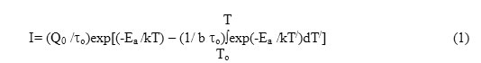
where Q_o is the total charge released during ITC run and is given by

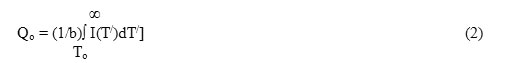
b is the constant linear heating rate according to the equation

T = T_o + bt                                 (3)

In eq. (3), T represents the absolute temperature corresponding to time t and T_o is the temperature where from ITC curve starts to appear. In eq. (1), τ_o is the fundamental relaxation time or the relaxation time at infinite temperature given by Arrhenius relation as ¹⁵

τ = τ_o exp( E_a/ kT )                      (4)

where τ is the relaxation time at T , k the Boltzmann’s constant and E_a the activation energy for the orientation of IV dipole.

The peak of the ITC spectrum appears at T_m such that

T_m² = {(b E_aτ_m)/ k}                    (5)

where τ_m is the relaxation time at T_m. It has been mentioned that eq. (1) corresponds to a TL glow curve involving first order kinetics, and hence TL glow curves involving higher order kinetics may also provide corresponding equations for ITC spectra. TL glow curves involving second and higher order kinetics have already been reported in the literature^16-18. Various efforts^19-21 have been made by different workers for the determination of dielectric relaxation parameters from ITC spectrum involving general order kinetics, but none of them have been found to be adequate when different order of kinetics are taken into consideration.

Keeping this aim in view, mechanisms responsible for the appearance of a ITC spectra are reconsidered in this article with an aim to establish a generalized equation. Detailed methods for the determination of dielectric relaxation parameters have been discussed.

Proposed Model of Analysis

In thermo luminescence, higher order kinetics has already been reported in the literature^16-18. Dwivedi et al¹⁸ has reported a new model for the occurrence of TL glow curve involving general orders kinetics. Orders of kinetics in thermo luminescence are dependent on the extent of recombination and simultaneous retrapping. Bucci, Fieschi and Guidi (BFG) method¹³ is usually employed to evaluate dielectric relaxation parameters E_a and τ_o in ITC measurements. Such evaluated values of dielectric relaxation parameters E_a and τ_o should satisfy eq. (5). However, it has been recorded that evaluated values of E_a and τ_o do not satisfy eq. (5) in general^19,22. This conclusion has been obtained at by Prakash and Nishad²², while developing characteristic relaxation time for a lattice dopant system.

Thus it has been observed that Eq. (5) is not adequate enough to explain the location of ITC spectrum of actual experimental systems. Keeping discussions of preceding paragraphs in view and in the light of the outcome of the model suggested by Dwivedi et al¹⁸ for TL glow curve involving general orders kinetics, a new model has been developed for the occurrence and analysis of ITC spectrum.

ITC spectrum

The thermally stimulated depolarization current density J depends on the rate of depolarization of IV dipoles and can be expressed as 

J = (-1/ℓ)dP(t)/dt                             (6 )

It has been found that the rate of depolarization depends on the remaining polarization P present at that time and on the relaxation time τ. In the present work it is proposed that the rate of depolarization also depends on the order of kinetics. Thus, the rate of depolarization can be expressed as

d P(t)/dt  = (-1/ℓ)[P(t) / t]             (7)

where ℓ is the order of kinetics involved in the system.

Eqn. (6) and (7) can be combined to have

J=(1/ℓ²)[P(t)/t]                                    (8)

Eqn.(7) after integration gives

P(t) = P_o exp [(-1/ℓ) (t / t) ]            (9)

where P_o is the maximum polarization. P₀ depends on polarizing electric field Ep and polarization temperature Tp as   

P_o =  [αN_d μ² Ep  / k Tp ]                 (10)

where N_d is the number of IV dipoles per unit volume each with dipole moment m, k the Boltzmann constant and a the geometrical parameter which for freely rotating dipoles has a value 1/3 (a equals to 2/3 for nn face centered vacancy positions in ionic crystals).

Eqn.(8) with help of eqns. (9) results into

J(t) =  [(1/ℓ²) P(t) /t]

= (1/ℓ²)(P_o/t) exp[-(1/ℓ)t /t]                 (11)

Non-isothermal form of eqn. (11) for the decay of polarization will be

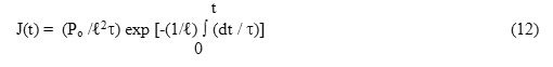
 where time is measured from the very appearance of the depolarization current after switching off the electric field. Use of the Arrhenius relation {eqn. (4)}, changes eqn.(12) into

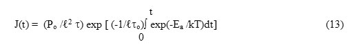
If the system is heated following a constant linear heating rate b as per eqn. (3). Then, eqn. (13) with the help of eqn.(3) can be re-arranged as

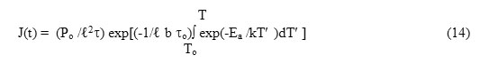
With the help of eqns.(1) and (14), one can write down the expression for the depolarization current  i (T) as

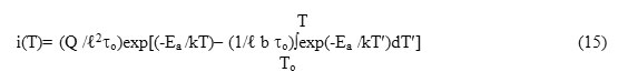
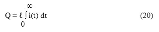
where Q is the total charge released in the ITC measurement and is related to P₀ through the relation

Q = P_o A = [αN_d μ² Ep A /k Tp ]                    (16)

where A is the cross sectional  area of  the  crystal specimen.

Equation (15) is the generalized equation for ITC spectrum involving ℓ th order of kinetics. Thus, it is obvious that one can have ITC spectra involving higher-order kinetics using eq. (15) after substituting the corresponding values of ℓ into it.

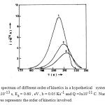
Some typical ITC curves as per eqn. (15) for different order of kinetics are shown in Fig. 1.

Click on image to enlarge

 Figure1: ITC spectrum of different order of kinetics in a hypothetical   system with t_o = 2.5×10-13 s, Ea = 0.60 , eV., b = 0.05 Ks-1 and Q =3×10-11 C. Number on the curves represents the order of kinetics involved.

Condition for the Peak of the ITC Spectrum

The condition for the occurrence of the peak of the ITC spectrum is obtained after differentiating eqn.(8) with respect to t and using eqn.(6) as

[(dJ/dt) t + J (dt/dt)] = (- J/ℓ)                 (17)

on putting the condition of maximum depolarization current in the ITC spectrum i.e. (dJ/dt)=0, we have from eqn. (17)

[ (dt_m/dt) + (1/ℓ)] J = 0

which suggest that either  

[(dt_m/dt)+ (1/ℓ)]  = 0 or J = 0

Since J can not be equal to zero in the range of temperature where ITC  spectrum is recorded, so it is obvious that

[(dt_m/dt) + (1/ℓ)] = 0 

this condition in combination with Arrhenius relation {eqn. (4) } gives

T_m²  =  [ℓb E_at_m / k] =(ℓt_o) (b E_a / k) exp[E_a / k T_m]                  (18)

where T_m is the temperature at which maximum current i_m in the ITC spectrum appears and t_m is the corresponding relaxation time at T_m. The values of T_m for different hypothetical systems are presented in table 1. It is obvious that T_m changes appreciably with a change in ℓ. Table 1 suggests that T_m remains unchanged for the same value of ℓt₀  in accordance with eqn. (18). Such a situation however, does not pose any problem in the evaluation of dielectric relaxation parameters. It is obvious from eqn.(18) that T_m is independent of Q and hence also of N_d as expected and appears to be at same location if b is kept fixed.

Table1: T_m for ITC Spectra for different sets of   E_a, ℓ and  t_o

Ea (eV)	to (s)	Tm   FOR (K)
		ℓ = 1	ℓ =  2	ℓ =  3
0.50	1.0 x 10-13	168	171	173
0.50	2.5 x 10-13	173	176	178
0.50	5.0 x 10-13	176	180	182
0.55	1.0 x 10-13	185	188	190
0.55	2.5 x 10-13	189	193	195
0.55	5.0 x 10-13	193	197	199
0.60	1.0 x 10-13	201	205	207
0.60	2.5 x 10-13	206	210	212
0.60	5.0 x 10-13	210	214	217
0.65	1.0 x 10-13	217	221	224
0.65	2.5 x 10-13	223	227	230
0.65	5.0 x 10-13	227	232	234
0.70	1.0 x 10-13	233	238	240
0.70	2.5 x 10-13	239	244	247
0.70	5.0 x 10-13	244	249	252

 

Evaluation of Dielectric Relaxation Parameters

From eqn.(6) one gets

i(t) =   (-1 /ℓ)dQ /dt                    (19)

Eqn.(19) after integration, can be rearranged as

and

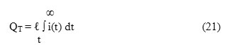
 If the system is heated as per eqn.(3) following a constant linear heating rate b, eqn.(21) changes as

where Q_T  is the number of released charge carriers per unit volume at the temperature T corresponding to  time t and A_T represents the area of the ITC spectrum enclosed within the temperature range T to ∞  such that

Further eqn.(20) can also be represented as

where A_o represents the total area enclosed within the ITC spectrum such that

Rearrangement of eqns.(11), (16) and (22), gives

X_T = ( ℓt_o )exp(E_a /kT)                (26)

where                                             

X_T  =  A_T / i(T)                   (27)

Eqn.(26) can further be written as

ln (X_T)= ln ( ℓt_o ) +(E_a /kT)                  (28)

For a given ITC curve of a system, ℓ, t_o and E_a are constant, so the plot of ln (X_T) vs  (1/T) will be a straight line with the slope (E_a /k) and  intercept equal to ln(ℓt_o). Such straight line plots in ln(X_T) vs (1/T) corresponding to Fig.1 is shown in Fig. 2.

Click on image to enlarge

 Figure2: Variation of ln [XT] Vs [1/T] for different order of kinetics in a hypothetical system with t0 = 2.5×10-13 s, Ea = 0.60 eV., b = 0.05 Ks-1 and Q =3×10-11 C. Number on the curves indicates the order of kinetics.

Thus, the activation energy can be evaluated from the slope of the straight line plot. The intercept gives the value of either ℓ or  t_o provided the other is known. In order to evaluate the order of kinetics involved we have calculated the value of the form factor g = (T_m/ (T₂–T_m)) similar to the case of TL processes¹⁸. The calculated values of form factor for different sets of E_a ,t_o and ℓ are listed in table 2.

Table2: Form factor for ITC spectra for different sets of E_a, ℓ and  t_o

Ea (eV)	to (s)	Form Factor  y = [Tm /(T2-Tm)]
		ℓ = 1	ℓ = 2	ℓ = 3
0.50	1.0 x 10-13	30.54	29.70	28.38
0.50	1.5 x 10-13	30.90	29.69	28.40
0.50	2.0 x 10-13	30.20	29.16	28.36
0.50	2.5 x 10-13	30.14	29.33	28.52
0.50	3.0 x 10-13	30.14	29.50	28.68
0.50	3.5 x 10-13	30.31	29.60	28.48
0.50	4.0 x 10-13	30.48	29.66	28.48
0.50	5.0 x 10-13	30.66	29.34	28.40
0.50	6.0 x 10-13	30.84	29.43	28.15
0.55	1.0 x 10-13	30.38	29.29	28.48
0.55	1.5 x 10-13	30.05	29.23	28.47
0.55	2.0 x 10-13	30.12	29.53	28.70
0.55	2.5 x 10-13	30.28	29.69	28.39
0.55	3.0 x 10-13	30.44	29.48	28.00
0.55	3.5 x 10-13	30.60	29.42	28.64
0.55	4.0 x 10-13	30.76	29.07	28.28
0.55	5.0 x 10-13	30.50	29.22	28.42
0.55	6.0 x 10-13	30.48	29.37	28.57
0.60	1.0 x 10-13	30.75	29.28	28.58
0.60	1.5 x 10-13	30.11	29.57	28.58
0.60	2.0 x 10-13	30.40	29.58	28.13
0.60	2.5 x 10-13	30.55	29.00	28.26
0.60	3.0 x 10-13	30.70	29.13	28.53
0.60	3.5 x 10-13	30.58	29.27	28.66
0.60	4.0 x 10-13	30.40	29.41	28.66
0.60	5.0 x 10-13	30.00	29.35	28.02
0.60	6.0 x 10-13	30.14	29.60	28.15
0.65	1.0 x 10-13	30.27	29.46	28.00
0.65	1.5 x 10-13	30.37	29.68	28.25
0.65	2.0 x 10-13	30.51	29.19	28.50
0.65	2.5 x 10-13	30.70	29.31	28.75
0.65	3.0 x 10-13	30.90	29.45	28.02
0.65	3.5 x 10-13	30.00	29.57	28.14
0.65	4.0 x 10-13	30.13	29.70	28.26
0.65	5.0 x 10-13	30.26	29.00	28.39
0.65	6.0 x 10-13	30.40	29.12	28.63
0.70	1.0 x 10-13	30.10	29.75	28.23
0.70	1.5 x 10-13	30.48	29.11	28.58
0.70	2.0 x 10-13	30.70	29.36	28.82
0.70	2.5 x 10-13	30.68	29.60	28.24
0.70	3.0 x 10-13	30.00	29.72	28.36
0.70	3.5 x 10-13	30.25	29.48	28.47
0.70	4.0 x 10-13	30.24	29.05	28.59
0.70	5.0 x 10-13	30.50	29.29	28.00
0.70	6.0 x 10-13	30.62	29.41	28.11
Average Value of form Factor		30.41	29.40	28.39

 

From the table 2 it is clear that the average value of form factor for first order kinetics is 30.41 and for second order kinetics it is 29.40 and for third order kinetics it is found to be 28.39.  To have the value of form factor γ justified for systems involving different order of kinetics 135 hypothetical systems have been considered in table 2. It should be mentioned that form factor γ for the systems involving first order kinetics as obvious from tables 2  lies  in the  range 30.00 ≤  γ  ≤  30.90,  and  that  for systems involving second order kinetics it lies in the range   29.00    ≤ γ ≤ 29.75   

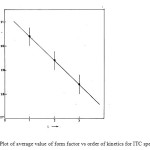
whereas for systems involving third order kinetics it is found to lie in the range 28.00   ≤ γ ≤ 28.82. A graph plotted between the average values of the form factor vs order of kinetics is shown in Fig 3.

Click on image to enlarge

 Figure3: Plot of average value of form factor vs order of kinetics for ITC spectrum.

From this curve, for a known value of form factor corresponding to an experimental ITC spectrum of a system, the order of kinetics involved can be ascertained. It should be noted that no overlapping values of form factor is obtained corresponding to different order of kinetics. The value of ℓ can also be determined using eqn.(24), if the value of N_d is known through some other independent experiment. Once the order of kinetics is known, the relaxation time can be evaluated from the intercept of the straight line plot drawn in accordance with eqn. (28). Thus the dielectric relaxation parameters E_a, ℓ and t_o can be evaluated in systems involving different order of kinetics.

Results and Discussion

The proposed model is free from all the anomalies discussed in the introduction section. A generalized equation is developed which is capable of explaining the occurrence and analysis of ITC spectrum involving different order of kinetics. While analyzing the ITC data reported in the literature ²², it has been found that eq. (5) is not satisfied. The values of dielectric relaxation parameters E_a and τ_o are evaluated ussing BFG method¹³ and are reported as such without taking care of eq. (5). However, It is essential that the evaluated values of E_a and τ_o must satisfy eq. (5). This aspect has not  been considered  by many researchers working in ITC studies. Keeping above facts in view a generalized equation has been developed which is capable of explaining the ITC spectrum involving different order of kinetics including first order. The anomalies associated with the eq. (5) have been removed through eqn. (18). Eqn. (18) for T_m gives the location of peak of ITC spectrum for different order of kinetics including first order. Figure 1 reveals that, peak position T_m shifts to higher temperature with a simultaneous decrease in the peak of the ITC spectrum i_m with increasing values of ℓ . It is obvious that change is more pronounced, when one goes from ℓ = 1 to ℓ = 2, which further decreases with increase in the  value of ℓ. The nature recorded in figure 1 is found to be in good agreement with eqs (15) and (18).

From factor g is found to be different for different ℓ. No overlapping values of g is found for different ℓ. Dielectric relaxation parameters are evaluated using straight line plots and hence errors if any during evaluation procedure are averaged out.

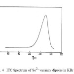
To seek acceptability and reliability of the proposed model it has been applied to a number of experimental systems whose ITC spectra are available in the literature. Experimental data of ITC spectra for a good number of systems have been utilized to evaluate the dielectric relaxation parameters following the suggested method of analysis. As a representative case suggested model has been applied to experimentally observed ITC spectra of KBr: Se2- system²³ which is shown in Fig. 4. The variation of ln (X_T) vs (1 / T) for KBr: Se2-  system is shown in Fig.5.

Click on image to enlarge

 Figure4: ITC Spectrum of Se2- vacancy dipoles in KBr system.

 

Click on image to enlarge

 Figure5: Plot of ln [XT] Vs [1/T] for KBr: Se2- system.

Evaluated dielectric relaxation parameters are presented in table 3. It is obvious from table 3 that there is good agreement in between reported and evaluated values of dielectric relaxation parameters.

Table3: Reported and evaluated values of dielectric relaxation parameters for KBr: Se2- system.

Reported				Evaluated
b(Ks-1)	ℓ	Ea (eV)	τo (s)	Form factor	ℓ	Ea (eV)	τo (s)
0.050	1(presumed)	0.720	2.00×10-14	30.60	1	0.718	1.99×10-14

 

It is worth mentioning that the KBr: Se2- system involves first order kinetics. Thus with the help of suggested model, one can evaluate successfully dielectric relaxation parameters namely activation energy E_a , fundamental relaxation time τ_o , order of kinetics ℓ and approximate number of dipoles per unit volume.

Conclusion

A generalized equation has been developed to explain the mechanisms responsible for the occurrence of the ITC spectrum involving different order of kinetics. Methodology has been developed to evaluate the dielectric relaxation parameters. The proposed model has been applied to number of experimental systems and it has been found that there is good agreement in between reported and evaluated values of dielectric relaxation parameters.

Acknowledgement

Author is thankful to Prof.  R. Chen   (Tel Aviv, Israil) and Prof. Jai Prakash, Ex Head, Department of Physics, D.D.U. Gorakhpur University, Gorakhpur for valuable suggestions during preparation of the manuscript.

References

1. Ikezaki, Fujite K , Wada I and Nakamura K  J,  J Electrochem Soc , 121, 591 (1974).
   CrossRef
   
2. Perlman M M , J  Electrochem Soc, 119, 892(1972).
   CrossRef
3. Wintle H J and Pepin M  P , J of Electrostat, 48, 115 (2000).
   CrossRef
4. Matsui K, Tanaka Y, Takada T, Fukao T, Fukunaga K, Maeno T and Alison J M,  IEEE Dielectr  Electr  Insul , 12, 406 (2005).
   CrossRef
5. Lee KY, Lee K W, Choi Y S, Park D H and Lim K J, IEEE Dielectr  Electr  Insul ,12, 566 (2005).
   CrossRef
6. Burghate P K, Deogaonkar V S, Sawarkar S B, Yawale S P and Pakade S V, Bull Matter Sc, 26, 267 (2003).
   CrossRef
7. Robert R, Barboza R, Ferreira G F L and Ferreira de Souza M , Phys Stat Sol, b 59, 335 (2006).
   CrossRef
8. Reichmanis E, Ober C K, McDonald  S, Iwaynagi T and  Nishikubo T, (Eds.) Microelectronics Technology: Polymers in Advanced Imaging and Packaging, American Chemical Society Symposium Series, 614(1995).
9. Yu S, Hing P and  Hu X, J Appl Phys, 88, 398 (2000).
   CrossRef
10. Ploss B, Shin F G , Chan H L W and  Choy C L,  Appl Phys Lett, 76, 2776 (2000).
    CrossRef
11. Patel K S, Kohl  P A and  Allen S A B, J Polymer Sc B Polymer Physics,38, 1634 (2000).
    CrossRef
12. Bucci C and  Fieschi R, Phys Rev Letters, 12, 16 (1964).
    CrossRef
13. Bucci C, Fieschi R and  Guidi G, Phys Rev, 148, 816 (1966).
    CrossRef
14. McKeever S W S , Thermoluminescence of Solids, Cambridge University Press, Cambridge (1988).
15. Arrhenius S Z, Z  Phys Chem,  4, 226 (1889).
16. Basun S, Imbusch G F, Jia D D and Yen W M, J lumen, 104, 283 (2003).
17. Prakash J, Solid   State   Comm,  85, 647 (1993).
    CrossRef
18. Dwivedi D K and Prakash J, Proc  Nat  Acad  Sci  India Sect A, 80, 153 (2010).
19. Prakash J , Pramana J Physics, 80, 143 (2010).
    CrossRef
20. Neagu R M and Neagu E R  , J Opto Electronics Adv Mat.,  8, 949 (2010).
21. Ahemad M T, J Korean Physical Society, 57, 272 (2010).
    CrossRef
22. Prakash J  and  Nishad A K , Japn J Appl Phys, 27, 2247 (1988).  
    CrossRef
23. Prakash J, J Phys, C12, L577 (1979).

---

This work is licensed under a Creative Commons Attribution 4.0 International License.