Abhishek Sharma1, Vishnu Prashad2 and Anil Kumar3
1Department of Energy, Maulana Azad National Institute of Technology, Bhopal, India.
2Department of Civil Engineering, Maulana Azad National Institute of Technology, Bhopal, India.
3Department of Energy, Maulana Azad National Institute of Technology, Bhopal, India.
DOI : http://dx.doi.org/10.13005/msri/080108
Article Publishing History
Article Received on : 09 Nov 2010
Article Accepted on : 11 Dec 2010
Article Published :
Plagiarism Check: No
Article Metrics
ABSTRACT:
This Paper Present a simulation for design of spear for nozzle by applying computational fluid dynamics analysis and using ANSYS software. With the development of high speed computers and advancement in numerical techniques detail flow analysis of the desired model can be done for design optimization. The design can be altered till the best performance or desired output is obtained. This is less time consuming.
CFD can provide the solution for different operating condition and geometry configuration in less time and cost and found very useful for design and development.
In the present work, three shapes of spear at different mass flow rates have been analysed using ANSYS-CFX 10 software, the pressure and velocity distribution are obtained and compared. Using the analysis result, the loss variations with the nozzles for different spear shapes are computed. The results are presented in tabular and graphical form.
KEYWORDS:
Numerical Modeling; Pelton wheel nozzle; Spear design
Copy the following to cite this article:
Sharma A, Prashad V, Kumar A. Numerical Simulation of Pelton Turbine Nozzle for Different Shapes of Spear. Mat.Sci.Res.India;8(1)
|
Copy the following to cite this URL:
Sharma A, Prashad V, Kumar A. Numerical Simulation of Pelton Turbine Nozzle for Different Shapes of Spear. Mat.Sci.Res.India;8(1). Available from: http://www.materialsciencejournal.org/?p=2475
|
Introduction
Hydraulic turbines have a series of blades fitted to wheel mounted on a rotating shaft.. Flowing water is directed on to the blades of a turbine runner, creating a force on the blade since the runner is spinning in this way energy is transferred from the water flow to the turbine The velocity and pressure of the liquid reduce while flowing through the hydraulic turbines.
This results in the development of torque and rotation of the turbine shaft. There are different forms of hydraulic turbines in use depending on the operational requirements. For every specific use, a particular type of hydraulic turbine provides the optimum output.
Classification of Hydraulic Turbines
Hydraulic turbines may be classified into various kinds on the basis of
The direction of flow of water
Pressure change
Head and quantity of water required
Position of the turbine shaft
Specific speed
Pelton Turbine
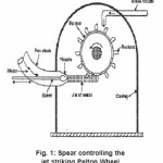
The Pelton wheel is among the most commonly used turbine for high head power plant. The Pelton wheel extract energy due to change of impulse (momentum) of moving water, as opposed to its weight like traditional overshot water wheel. Although many variations of impulse turbines existed prior to Pelton design, they were less efficient than Pelton’s design, the water leaving these wheels typically still had high speed, and carried away much of the energy. Pelton’ paddle geometry was designed so that when the rim runs at ½ the speed of the water jet, the water leaves the wheel with very little speed, extracting almost all of its energy, and allowing for a very efficient turbine. The runner consists of a circular disk with a buckets evenly spaced round its periphery. The buckets have a shape of double semi-ellipsoidal cups. Each bucket is divided into symmetrical parts by a sharp-edged ridge known as splitter.
Figure 1: Spear controlling the jet striking Pelton Wheel
Principles of Fluid Flow
There are three basic principles of fluid flow
Principle of Conservation of Mass
It states that “Mass can neither be created nor destroyed”. Continuity equation has been derived on this principle.
Principle of Conservation Of Energy
It states that “Energy can neither be created nor destroyed”. On the basis of this principle the energy equation is derived.
Principle of Conservation of Momentum
It states that “The impulse of the resultant force, or the product of the force and time increment during which it acts is equal to change in momentum of the body”. Momentum equation is derived on this basis.
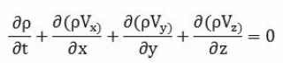
Continuity Equation
The rate of increase of the fluid mass contained within the region must be equal to the difference between the rate at which the fluid mass enters the region and the rate at which the fluid mass leaves the region. However, if the flow is steady, the rate of increase of fluid mass within the region is equal to zero, then the rate at which the fluid mass enters the region is equal to the rate at which the fluid mass leaves the region.
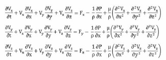
Momentum Equation
According to Newton’s Second Law of motion, inertia force acting on a body in any direction is equal to resultants of all body and surface forces in that direction.
Energy Equation
Energy equation is obtained by multiplying the equation of momentum by velocity components in each coordinate direction and then adding and integrating over the volume
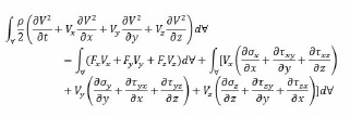
Flow Through Nozzle
A nozzle is a gradually converging short tube which is fitted at the outlet and of the penstock for the purpose of converting the total energy of the flowing water into kinetic energy. Nozzles are used where high velocities of flow are required to be developed. In impulse turbines, it is required to convert whole of hydraulic energy into kinetic energy.
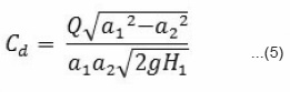
The discharge is given by,
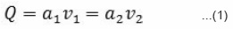
The nozzle is horizontal and the nozzle axis is assumed as datum for elevation and hence head at nozzle is given by,
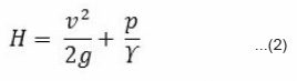
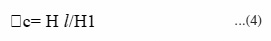
Head loss in nozzle is given by,
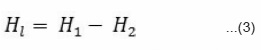
Head loss coefficient is given by,
Coefficient of discharge is given by,
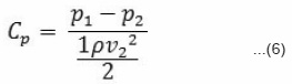
Coefficient of pressure is given by,
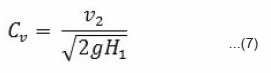
Coefficient of velocity is given by,
Computational Fluid Dynamics
Computational fluid dynamics (CFD) is one of the branches of fluid mechanics that uses numerical methods and algorithms to solve and analyze problems that involve fluid flows. Computers are used to perform the millions of calculations required to simulate the interaction of liquids and gases with surfaces defined by boundary conditions. Even with high-speed supercomputers only approximate solutions can be achieved in many cases. Ongoing research, however, may yield software that improves the accuracy and speed of complex simulation scenarios such as transonic or turbulent flows. Initial validation of such software is often performed using a wind tunnel with the final validation coming in flight test.
Geometric Modeling
Modeling
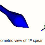
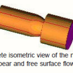
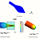
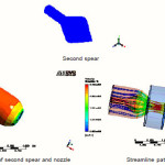
The modeled assembly of nozzle for pelton turbine consists of nozzle (pipe of converging cross-sectional area), spear and a free surface flow domain. The modeled assembly consists of inlet, nozzle, spear and outlet. The modeled assembly of free surface flow domain consists of extended outlet. The modeling has been done in ANSYS Workbench 10 and ANSYS ICEM CFD 10. The 3D-view of spear is shown in fig.
Figure 2
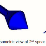
Figure 3
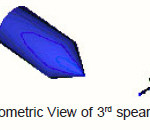
Figure 4
Figure 5
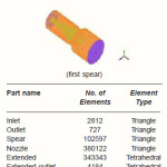
Table 1: Mesh Data for Nozzle Spear Domain
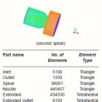
Table 2: Mesh Data for Nozzle Spear Domain
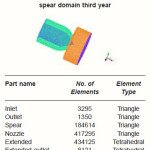
Table 3: Mesh data for nozzle spear domain third year
Mesh generation
The geometry made is divided into small sub parts for CFD analysis called mesh and the process is called meshing. The shape of the mesh elements can be triangular, quadrilateral, tetrahedral, hexahedral or prism depending upon the size and shape of the geometry. The shape and size of the mesh elements can be varied and are kept according to the dimension of the geometry, accuracy required, computational power of the system and memory. The complete nozzle flow space is divided into two domains and the mesh is generated.
The meshing of nozzle and spear domain has been done at different spear shapes and the meshing of nozzle spear domain for fillet spear shape has been shown in fig.
The summary of meshing data for each surface has been described in table
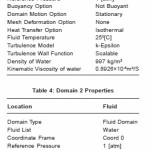
Domain And Interface Properties
The mesh is converted into the required format and is imported to ANSYS CFX-10 software. In ANSYS CFX-Pre the properties of the domains and fluid are defined along with their interface properties. The summary of the domain 1 properties are given in table 5.13.
Boundary Conditions
The boundary conditions are applied at the inlet and outlet surfaces of the domains.
Inlet Boundary Condition
The mass flow rate and its direction with normal direction to the inlet surface i.e., at inlet of nozzle domain is applied. Turbulence is set to medium intensity (upto 5%).
Outlet Boundary Condition
The reference pressure at the outlet of the external domain was set equal to 1 atmospheric.
Wall Conditions
The walls of all the domains are assumed to be smooth and no slip condition is assigned.
Turbulence Model: k- C model used
Table 4: Domain 1 Properties
Solver
Specific Blend Factor with 0.9 value has been used for up to 200 iterations. The timescale control is set to Auto Timescale. The RMS residual target has been set to 1x10E-7 for termination of the calculations.
Post Processing
3D-Streamlines of velocity and pressure contours starting from inlet of the nozzle can be seen in all the domains. Using the function calculator in tools average values of various parameters like the velocity, pressure, area, mass flow rate at the boundaries and the required domain can be found out for computation of loss, pressure and velocity coefficients.
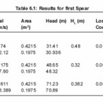
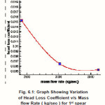
The outlet velocity and the head loss increases with the increase in mass flow rates for the same spear as seen in Tables 6.1. The head loss coefficient decreases gradually as mass flow rate for spear increasing from 3952.12 kg/sec to to 4940.15 kg/sec as seen in Fig.6.1
The coefficient of discharge has least value at mass flow rate of 5928.18 kg/s .and coefficient of velocity have least value at mass flow rate 3952.12 kg/sec
Coefficient of pressure decreases with increase in mass flow rate from 2412.74 kg/sec to 3619.11 kg/sec.
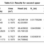
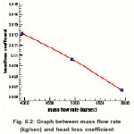
Head loss increases with increase of mass flow rates for the second spear as seen in Tables 6.2 It is maximum at 4940.15 kg/sec mass flow rate and start decreases when mass flow rate increasing to 5928..18 kg/sec . head loss coefficient start decreasing as mass flow rate increasing, as shown in fig 6.2.
Coefficient of velocity increases as the mass flow rate are increases it it 0.8098 at 3952.12 kg/sec and increases to 0.8107 when mass flow rate increases to 4940.15 kg/sec and again increases to 0.8116 when mass flow rates increases to 5928.18 kg/sec .
Coefficient of pressure decreases gradually as mass flow rate are increses it is o.9608 when mass flow rate is 3952.12 kg/sec and decreases to 0.9598 when mass flow rate increases to 4940.15 kg/sec and again decreases to 0.9596 when mass flow rate increases to 5928.18 kg/sec .
Coefficient of discharge decreases as the mass flow rate increses gradually it is max for mass flow rate 3952.12 kg/sec and minimum for mass flow rate 4940.15 kg/sec .and by increasing mass flow rate to 5928.18 kg/sec it is partially increases as from 0.67038 to 0.6706.
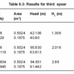
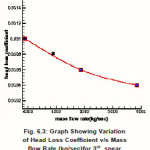
Head loss increases with the increase in mass flow rates for the spear as seen in Tables 6.3 and Head loss coefficient decrease when mass flow rate increasing from 3952.12 kg/sec to 5928.18 kg/sec from 0.0310 to 0.0304 respectively .
Coefficient of velocity decreases as mass flow rate increases from 3952.12 kg/sec to 5928.18 kg/sec.
Coefficient of pressure decreases as mass flow rate increases from 3952.12 kg/sec to 5928.18 kg/sec.
Coefficient of discharge increases gradually from 3952.12 kg/sec mass flow rate to 4940.15 kg/sec as from 0.6404 to 0.64094 and it is decrease when mass flow rate increases to 5928.18 kg/sec to 0.64093.
Table 6.1: Results for first Spear
Table 6.2: Results for second spear
Table 6.3: Results for third spear
Figure 6.1: Graph Showing Variation of Head Loss Coefficient v/s Mass flow Rate ( kg/sec ) for 1st spear
Figure 6.2: Graph between mass flow rate (kg/sec) and head loss coefficient
Figure 6.3: Graph Showing Variation of Head Loss Coefficient v/s Mass flow Rate (kg/sec)for 3rd spear
Graphical Plots
Pressure contours and velocity stream lines were obtained using insert contour and insert streamline commands of menu bar in ANSYS CFX-Post. Pressure contours and velocity stream lines for each geometry at different spear shape varying mass flow rate has been shown under.
Figure 7
This streamline flow shows that after nozzle outlet streamline start conversing to a point that is vina contracta and after that streamline start spreading, in the inner region red stream line shows higher pressure and uniformly distribution of streamline shows high velocity and in the outlet part of free surface domain streamline are not uniformly distributed that shows less velocity and yellow and green line streamline shows less pressure distribution shown in Fig.
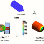
Figure 8
In this fig streamline after nozzle outlet start converging that shows increasing the velocity, and in the outer periphery of extended domain it is not evenly distributed that is showing less velocity, and red color of streamline showing higher pressure distribution in the middle of extended domain. shown in Fig.
Figure 9
At the outlet of nozzle strip of blue color shows less pressure distribution and it is increasing towards inlet of nozzle,difference between this and previous nozzle spear domain is that in this case pressure is suddenly increasing and long area of red strip shows that pressure is high in most of the part of nozzle
Conclusion
In this dissertation Computational Fluid Dynamics (CFD) approach has been used to predict the performance of different shape of spear at different mass flow rates and nozzle openings.
The pressure at the inlet of the nozzle and spear increases with the increase in mass flow rate for the same spear shape .The pressure is maximum for the second spear and nozzle geometry at the 5928.18 kg/sec mass flow rate at the inlet and it is minimum for the first spear and nozzle with 3952.12 kg/sec mass flow rate.
The pressure at the outlet is nearly equal to atmosphere as the jet is issued freely in air. The outlet velocity of the jet is higher than the inlet velocity of the fluid which shows that the pressure energy is being converted into kinetic energy.
The coefficient of pressure is max for second spear (0.9608) having mass flow rate 3952.12 kg/sec.
The velocity increases with the increase in mass flow rates from 3952.12 to 5928.18 kg/sec at the inlet and at the outlet for all spear because of constant area.
The coefficient of velocity is maximum for the first spear (0.8998) having 4940.15 kg/sec mass flow rate.
The coefficient of discharge is maximum for the first spear (0.789755) having 4940.15 kg/ sec mass flow rate.
The streamlines converge slowly for third shape spear nozzle geometry but for second and first spear nozzle geometry streamlines converge sharply as these has sharp curvature as seen in Figures
Due to sharp curvature, the pressure at outlet of the third spear nozzle geometry is more than the pressure at outlet of the first and second spear geometry.
The third spear nozzle geometry has the highest head loss coefficient (0.0310) among all the three geometry.
From the streamlines, it is seen that the jet coming out of 1st and 2nd spear and nozzle diverges as seen in Figure but the jet coming out of 3rd spear nozzle remains compact as seen in Figures (Vena-contracta can be seen in velocity streamlines when the jet of water just leaves the nozzle as seen in Figures)
The computation and comparison of different flow coefficients of various geometric configurations using CFD will help to optimize the nozzle and spear shape.
In present case it may be concluded that 1st spear is better than the other two spears.
Pressure Distribution Across Cross Section Area
It is observed that pressure is highest at inner periphery and decreases towards outer side,
The pressure distribution on a plane at the highest curvature point of spear shows that pressure is minimum at the inner periphery and increases towards outer periphery.
It is also seen that as the mass flow rate increases pressure values at any point on any cross section area increases.
References
- W.A.Doble, “The Tangential Water Wheel”,Transaction of the American Institute of Mining Engineers, 29, 852-858 (1899).
- W Malalasekera and H K Versteeg, “An Introduction to Computational Fluid Dynamics”, the Finite Volume Method, Longman (1995).
- W.N. Dawes, “Computational Fluid Dynamics for Turbomachinery Design”, Whittle Laboratory, Department of Engineering,University of Cambridge, UK (1998).
- Kearon Bennet, Jacek Swiderski, Jinxing Huang, “Application of CFD Turbine Design for Small Hydro Elliott Falls, A Case Study”,Transaction of SECFD, Ottawa engineeringlimited, Ottama, Ontario (2000).
- Eisinger R, Ruprecht A., “Automatic Shape Optimization of Hydro Turbine Components Based on CFD”, Transaction of Emeraldinsight, 6(1): pp.101-111 (2001).
- Maryse Francois, Pie Yves Lowys, Gerard Vuillerod, “Development and Recent Projects for Hooped Pelton Turbine”, Transaction of HYDRO-2002, Turkey, Alstorm (2002).
- Yodchai Tiaple, Udomkiat Nontakaew, “The Development of Bulb Turbine for Low Head Storage Using CFD Simulation”, Transaction of ENERGY-BASED.NRTC.GO, publication #1, pp.10-14
- B. Zoppe, C. Pellone, T. Maitre, P. Leroy, “Flow Analysis Inside a Pelton Turbine Bucket”,Transaction of ASME, 128: 500-511 (2006)
CrossRef
- Michael Marek, Thorsten Stoesser, Philip J.W. Roberts, Volker Weitbrecht, Gerhard H.Jirka, “CFD Modelling of Turbulent Jet Mixingin a Water Storage Tank”, Transaction of UNIKARLSRUHE,pp.1-10 (2006).
- Zn Zhang , M Casey , “Experimental Studiesof the jet of a Pelton Turbine”, Power and Energy , Mech E Vol. 221 Part A, pp.1181-1189
- Bansal R.K., “A textbook of Fluid Mechanics and Hydraulic Machines”, Laxmi Publications, New Delhi (2005).
- S Bharat Krishna and Prof V Ganeshan,“CFD Analysis of Flow through vane swirlers”
- Paul Breeze, “Hydropower: Power Generation Technologies”, pp. 104-121(2005).
- Peggy Brookshier, “Hydropower Technology”,U.S. Department of Energy, Idaho, United States (2005).
- Shamesw I.H., “Mechanics of Fluids”,McGraw Hill Publications (2002).
- Roer E.A. Arndt, “Hydroelectric Power Stations”, Encyclopaedia of Physical Science and Technology, pp. 489-504 (2005).
- www.springerlink.com
- http://scitation.aip.org
- http://www.mathematik.uni-dortmund.de
- ANSYS, 2005, CFX-10.0, user manual
- User manual from fluent.com

This work is licensed under a Creative Commons Attribution 4.0 International License.