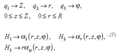
as the generalized cylindrical coordinates, and below it is convenient to redesignate:
of pores, not depend on z. Since for the rectilinear cylindrical coordinates
from the usual cylindrical.
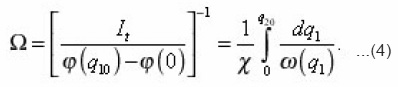
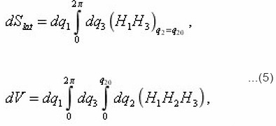
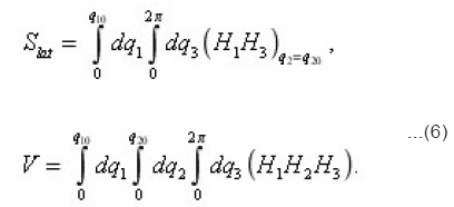
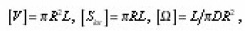
the characteristics of individual pore (4)-(6) after utilizing dimensionless coordinates with the aid of the scales
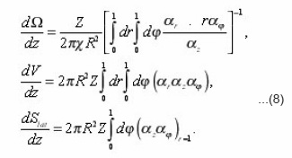
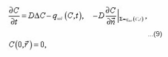
The method of eigenvalue coordinates of pores allows to obtain the transport equations in a single pore, expressing its coefficients through the local parameters (8). Let us for this purpose consider, for example, the diffusion of the components of the solution with the concentration in the liquid pores, determined in the general case by boundary-value problem
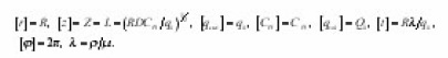
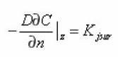
-normal to the interphase boundary Σ. The equation (9) is now to carry on an individual i pore, assuming Σ its lateral surface. In Σ its eigenvalue coordinates r, z, φ, are made dimensionless using the scale
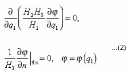
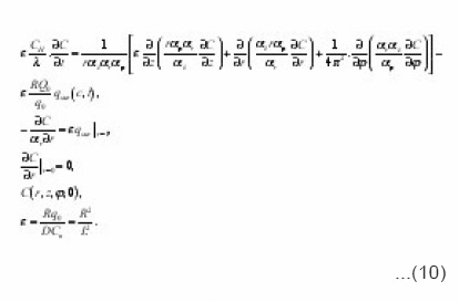
The problem (9) is written in the form of (index i, r, z, φ and other variables, are omitted for brevity, it is assumed):
The conjugation conditions at the border with neighboring pores is expected to be met. If all the terms are multiplied by a factor
integrated by the coordinates and take into account the boundary conditions , then (10) is reduced to use in the future as an integral form
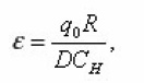
In the equation (10), the parameter ε is equal to the ratio of the characteristic scales of absorption flow q0 on the boundary surface and diffusion,
But L is interpreted as the depth of penetration of diffusion into the volume of the environment. Since it is assumed that the substance is transferred through entire pore space, then and are small q0 and ε respectively
(Otherwise, the limit within one pore, absorption almost complete). Therefore in (10) it is possible to use a perturbation theory and to represent C ( r,z,φ,0)
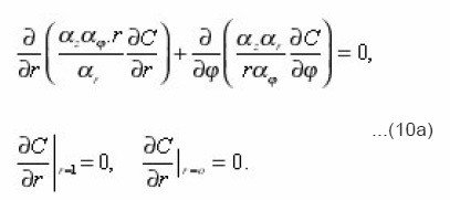
with a series in powers of small parameter . Then in the zero by approximation, on the basis of (10),
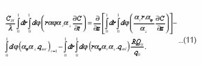
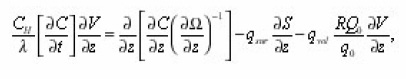
Physically necessary solution of the equation (10 a) is an arbitrary function C = C ( t,z) of time and eigenvalues coordinate z. It simultaneously satisfies the equation (11) which is due to the independence of C on r and Φ is simplified:
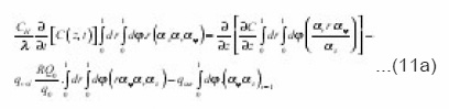
Coefficients (11a) coincide with the integrals (8), and if we make

dimensionless with the aid of the scales
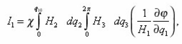
then (11) is led to the formula:
or in the dimensional form:
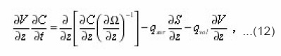
Thus, it is possible to establish, that the equation (12), which expresses the balance of substance in the volume dv of a certain pore, connected the transport process with its local characteristics. This gives the possibility to consider the problems, complicated by the presence of mobile interphase boundary and to express the effective transport coefficients through the integral characteristics of environment. Let’s proceed with expressions (8) for local parameters
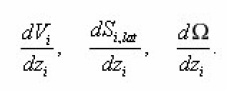
Preliminarily let us pass, using determination of sinuosity
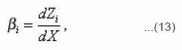
from z to the homogeneous coordinate x , on which all depend macroscopical, i.e. the averaged values. In a case of plane-parallel medium considered below the axis is perpendicular to its surface and
Where zi, x – dimensional, and therefore Z is absent.
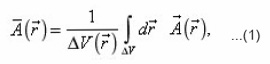
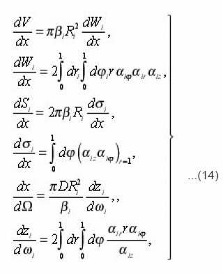
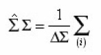
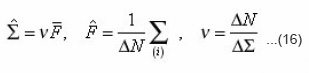
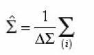
For the calculation g, sud, xef it is necessary to average (14) with the aid of the rule
(1), and since Vi, Si are volume and surface of pores, then as a result of their averagings we will obtain g and sud As the volume of averaging Δv = ΔΣ. Δx let us select infinitely thin layer ( x, x+ Δx ) with the area of base ΔΣ and will act on the equation (2) by the operator
Summation over all N(x) pores of the layer. Then on the left side we obtain:
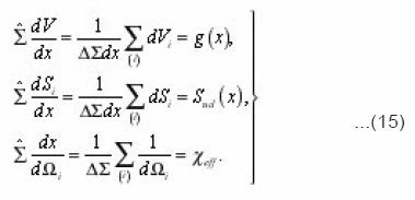
To the right in (14) it is convenient to represent
It is obvious, that is equal the density of pores, which intersect layer ( x, x + dx ) At
formula
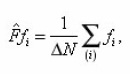
determines mean-static

on the infinite ensemble of pores of section. From this point of view, by the force of limitation ΔΣ use (16) gives, strictly speaking, an average on a certain sample ΔN from this ensemble, and the density can fluctuate. However, since the probability of deviations from f is proportional 1/ΔN, and

then the below noted difference is ignored. From (14), (15) we find

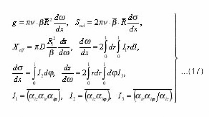
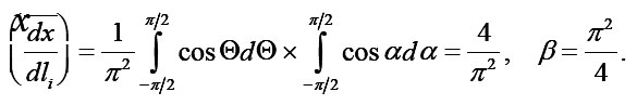
Calculating l123 , taking into account that

they characterize the curvatures of arcs in the generalized coordinate system relative to the appropriate arcs of the usual cylindrical system (where αz=αr=αφ=1).
In the chaotic porous space, these curvatures are independent for different directions, so that
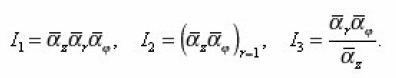
At the same time, as a result of uniformity of medium along the section ΔΣ and complete chaos in the geometry of pores, any deviations from one are equally probable and consequently
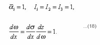
If dispersions D(R) and D(β) are small, then
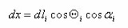
νdlDxz, dl r , dlϕ
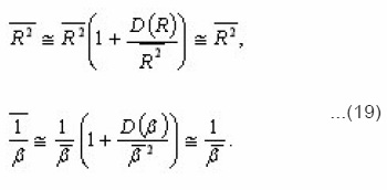
And by the force of (17)-(19), we obtain
Thus, five integral characteristics g, sud, xeff, v, β, R , are bound by three relations (20). From them, in particular, follow the equalities
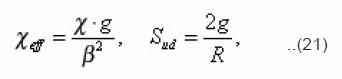
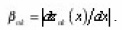
which in the general case of arbitrary environment were not obtained. For the problems of electrical conductivity the diffusion coefficient in (20) is substituted by the coefficient of electrical conductivity χ. Sinuosity β is found from the determination of arc length dli=αizdzi..
Actually, since
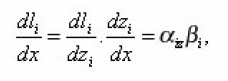
Where
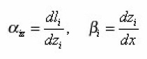
Then, averaging this equation over an ensemble of pores, we have
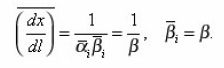
Since
(Where-

the Directing angles of the arcs dli ) and averagings over the ensemble and all orientations of arcs relative to axis are equivalent, then
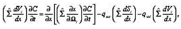
With the aid of that used above for calculating (20) the procedure it is possible to average the equation of diffusion in the separate pore. In the beginning in (12) we will pass from eigenvalues to the homogeneous coordinate.Then we obtain taking into account (13)
On both parts of (20), let us act by the operator of summation
and let us consider that the concentration Ci(x) must weakly depend on index i, i.e., the number of pore in the section ΔΣ. This is a consequence of connectivity and cross-pore space. Owing to the fulfillment of conditions for conjugation in the points of small intersections of the root-mean-square spread σ of values Ci(x), caused by difference in the geometry of the pores of layer (x,x+dx) and their previous branchings (see below). Therefore all values, connected with Ci(x) it is possible to carry out from the summation sign and then from (22) we find
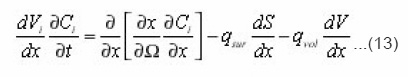
Where qsur and qvol have already the sense of averages by volume ΔΣdx density of sources. Hence, taking into account (15) we finally obtain the required equation for the averages
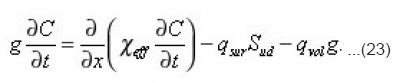
The presented method makes it possible to derive in the subsequently equations, analogous (23), in the case of mobile interphase boundary. The diffusion of the components of the solution in the porous medium, accompanied by their crystallization on the pore walls, can serve as its example.
Let us return to evaluation quantity
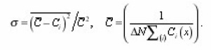
For this it is expedient to consider the simplest model, which assumes all intersections with those (!!!!) located in the planes xn = λn. where n=1,2,3…,β0λ- the average length of the pores. Furthermore, let us accept their radii Ri sinuosity βi as that being independent of x, and the probability of branching and confluence (merging) in each plane equal. Then, using expressions forthe concentrations at the nodal points 
which appear from equations of diffusion, also of conjugating conditions, it is possible to show that
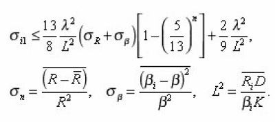
Summing up is here produced with the aid of

On the Boundary x=0 , (corresponding n=0) ) all concentrations
are equal and, consequently

The parameter in the expression defines the flow to the surface of the pore
And the depth of penetration of diffusion into the porous environment is assigned.
And since it is great in comparison with the length of pore

then σ is small and, therefore, Ci is weakly depends on i.Further let us pause in greater detail at the determination of sinuosity β(x). Formula (13) assumes that, β – the single-valued function of homogeneous coordinate x . However, this condition is disrupted, if a certain part of the pores had turning points, so that they intersect layer (x, x +dx) several times in opposite directions (in the chaotic pore space the probability of this it is certain, it is small). Then procedure presented above necessary to generalize, since the flow of diffusion current for-branching pore corresponds to the series, but not parallel connection of its elements of those belonging to the allocated layer (x, x +dx) and this influences the calculation of

moreover sinuosity
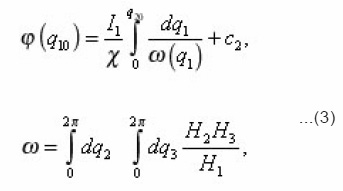
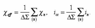
Considering for simplicity the case of absence the sources, it is easy to show that the average for all-branches of the pore concentration value satisfies the equation
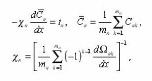
Where- the current through the pore. According to its meaning is the conductivity of the layer of unit thickness, containing a single pore. Therefore it is clear that effective conductivity
Acting by the operator of summing up S to both parts of (12) again, we come to the homogeneous equation
analogous (11). Summarizing the state that the above obtained relations connecting the effective transport coefficients with the structure of an arbitrary porous environment. A general method is developed, which allows to obtain in different cases the homogeneous transport equation.
References
- Color R., and others. Optical holography.V. 1. – Moscow: MIR. – 1973.
- Komotskii V. A., Black T. D. Analysis and application of stationary reference grating method for optical detection of surface acoustic waves // J. Appl. Phys.- V. 52 (January 1981).
CrossRef
- Kaufman M., Seidman A. Handbook of electronics calculation for engineers and technicians. McGraw-Hill, New York, 1988 ISBN 5-283-02512-8 (V.2, Russ.) ISBN 5- 283-02506-3 (Russ.) ISBN 0-07-033528-1 (Eng.).
- Oliner A., edited by. Surface acoustic waves.- Moscow: MIR.- 1981.
- Komotskii V. A., Application of methods of three-dimensional frequency response analysis for the solution of some problems of coherent optics.- Moscow: RFU.-1994.
- Bessonov A. F., and others. Measurement of the phase distributions of surface acoustic waves by the method of optical sounding with the supporting diffraction of the lattice // Autometry.5 (1982).
- Deryugin l. N., and others. Practical realization of the phase measurements of surface acoustic waves at optical sounding with the supporting diffraction of the lattice // Autometry. 3 (1988).
- Bessonov A. F., and others. Optical sounding of surface acoustic waves in the presence of stationary periodic lattice // Optics and spectroscopy. V. 49(1980).
- Bessonov A. F., and others. Interaction analysis of light wave with the system of the three-dimensional diverse periodic structures during the optical sounding of surface acoustic waves // Optics and spectroscopy.- V. 56(1984).
- Komotskii V. A., et al. An optical setup for measuring amplitude and phase distributions of surface acoustic waves // Instrument and experimental techniques. V. 41(1998).
- Kaschenko N. M., Komotskii V. A. On November 23-25, 1999. – The measurement of rectangular periodic structures with the aid of the laser sounding. – the 6th All-Russian scientific and technical conference “State and the problem of the measurements” Theses of reports, the second part. Moscow.
- Komotskii V. A. On May 19 to 22, 1998. – The improvement of the optical method of determining the depth of the periodic structures.- 34 scientific conference of the faculty of physical-mathematical and natural sciences. Moscow: RFU.- Theses of reports, physical sections, the publishing house of the Russian friendship university, p.29 (1998).
- Kaschenko N. M., Komotskii V. A. On May 24 to 28, 1999. – measurement of the depth of supporting diffraction of lattices at a deviation of the form from meander.- Theses of reports, physical sections. Moscow: RFU.
- Komotskii V. A. Characteristic and the possibilities of a method of the optical sounding of surface acoustic waves with the use of supporting diffraction lattices // Bulletin RFU.- V. 1 (1993).
- Kaschenko N. M., Komotskii V. A. Phase measurements of wave fields of surface acoustic waves by a method of optical sounding with the use of supporting diffraction lattices // Bulletin RFU.- V. 1 (1998).